This blog post is written by AI CDT student, Jonathan Erskine
I recently attended the ELISE Wrap up Event in Helsinki, marking the end of just one of many programs of research conducted under the ELLIS society, which “aims to strengthen Europe’s sovereignty in modern AI research by establishing a multi-centric AI research laboratory consisting of units and institutes distributed across Europe and Israel”.
This page does a good job of explaining ELISE and ELLIS if you want more information.
Here I summarise some of the talks from the two-day event (in varying detail). I also provide some useful contacts and potential sources of funding (you can skip to the bottom for these).
Robust ML Workshop
Peter Grünwald: ‘e’ is the new ‘p’
P-values are an important indicator of statistical significance when testing a hypothesis, whereby a calculated p-value must be smaller than some predefined value, typically $\alpha = 0.05$. This is a guarantee that Type 1 Errors (where null hypothesis can be falsely rejected) are less than 5% likely.
“p-hacking” is a malicious practice where statistical significance can be manufactured by, for example:
- stopping the collection of data once you get a P<0.05
- analyzing many outcomes, but only reporting those with P<0.05
- using covariates
- excluding participants
- etc.
Sometimes this is morally ambiguous. For example, imagine a medical trial where a new drug shows promising, but not statistically significant results. Should a p-test fail, you can simply repeat the trial, sweep the new data into the old and repeat until you achieve the desired p-value, but this can be prohibitively expensive, and it is hard to know whether you are p-hacking or haven’t tested enough people to prove your hypothesis. This approach, called “optional stopping”, can lead to violation of Type 1 Error guarantees i.e. it is hard to have faith in your threshold $\alpha$ due to the increasing cumulative probability that individual trials are in the minority case of false positives.
Peter described the theory of hypothesis testing based on the e-value, a notion of evidence that, unlike the p-value, allows for “effortlessly combining results from several studies in the common scenario where the decision to perform a new study may depend on previous outcomes.“
Unlike with the p-value, this proposed method is “safe under optimal continuation with respect to Type 1 error”; no matter when the data collecting and combination process is stopped, the Type-I error probability is preserved. For singleton nulls, e-values coincide with Bayesian Factors.
In any case, general e-values can be used to construct Anytime-Valid Confidence Intervals (AVCIs), which are useful for A/B testing as “with a bad prior, AVCIs become wide rather than wrong”.
In comparison to classical approaches, you need more data to apply e-values and AVCIs, with the benefit of performing optional stopping without introducing Type 1 errors. In the worst case you need more data, but on average you can stop sooner.
This is being adopted for online A/B testing but is more challenging for expensive domains, such as medical trials; you need to reserve more patients for your trial, but you wont need them all – a challenging sell, but probability indicates that you should save time and effort in the majority of cases.
Other relevant literature which is pioneering this approach to significance testing is Waudby-smith and Ramdas, JRSS B, 2024
There is an R package here for anyone who wants to play with Safe Anytime-Valid Inference.
Watch the full seminar here:
https://www.youtube.com/watch?v=PFLBWTeW0II
Tamara Broderick: Can dropping a little data change your conclusions – A robustness metric
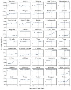
Tamara advocated the value of economics datasets as rich test beds for machine learning, highlighting that one can examine the data produced from economic trials with respect to robustness metrics and can come to vastly different conclusions than those published in the original papers.
Focusing in, she described a micro-credit experiment where economists ran random controlled trials on small communities, taking approximately 16500 data points with the assumption that their findings would generalise to larger communities. But is this true?
When can I trust decisions made from data?
In a typical setup, you (1) run an analysis on a series of data, (2) come to some conclusion on that data, and (3) ultimately apply those decisions to downstream data which you hope is not so far out-of-distribution that your conclusions no longer apply.
Why do we care about dropping data?
Useful data analysis must be sensitive to some change in data – but certain types of sensitivity are concerning to us, for example, if removing some small fraction of the data $\alpha$ were to:
- Change the sign of an effect
- Change the significance of an effect
- Generate a significant result of the opposite sign
Robustness metrics aim to give higher or lower confidence on our ability to generalise. In the case described, this implies a low signal-to-noise ratio, which is where Tamara introduces her novel metric (Approximate Maximum Influence Perturbation) which should help to quantify this vulnerability to noise.
Can we drop one data point to flip the sign of our answer?
In reality, this is very expensive to test for any dataset where the sample size N is large (by creating N*(N-1) datasets and re-running your analysis. Instead, we need an approximation.
Let the Maximum Influence Perturbation be the largest possible change induced in the quantity of interest by dropping no more than 100α% of the data.
From the paper:
We will often be interested in the set that achieves the Maximum Influence Perturbation, so we call it the Most Influential Set.
And we will be interested in the minimum data proportion α ∈ [0,1] required to achieve a change of some size ∆ in the quantity of interest, so we call that α the Perturbation-Inducing Proportion. We report NA if no such α exists.
In general, to compute the Maximum Influence Perturbation for some α, we would need to enumerate every data subset that drops no more than 100α% of the original data. And, for each such subset, we would need to re-run our entire data analysis. If m is the greatest integer smaller than 100α, then the number of such subsets is larger than $\binom{N}{m}$. For N = 400 and m = 4, $\binom{N}{m} = 1.05\times10^9$. So computing the Maximum Influence Perturbation in even this simple case requires re-running our data analysis over 1 billion times. If each data analysis took 1 second, computing the Maximum Influence Perturbation would take over 33 years to compute. Indeed, the Maximum Influence Perturbation, Most Influential Set, and Perturbation-Inducing Proportion may all be computationally prohibitive even for relatively small analyses.
Further definitions are described better in the paper, but suffice to say the approximation succeeds in identifying where analyses can be significantly affected by a minimal proportion of the data.For example, in the Oregon Medicaid study (Finkelstein et al., 2012), they identify a subset containing less than 1% of the original data that controls the sign of the effects of Medicaid on certain health outcomes. Dropping 10 data points takes data from significant to non-significant.
Code for the paper is available at:
https://github.com/rgiordan/AMIPPaper/blob/main/README.md
An R version of the AMIP metric is available:
https://github.com/maswiebe/metrics.git
Watch a version of this talk here:
https://www.youtube.com/watch?v=7eUrrQRpz2w
Cedric Archambeau | Beyond SHAP : Explaining probabilistic models with distributional values
Abstract from the paper:
A large branch of explainable machine learning is grounded in cooperative game theory. However, research indicates that game-theoretic explanations may mislead or be hard to interpret. We argue that often there is a critical mismatch between what one wishes to explain (e.g. the output of a classifier) and what current methods such as SHAP explain (e.g. the scalar probability of a class). This paper addresses such gap for probabilistic models by generalising cooperative games and value operators. We introduce the distributional values, random variables that track changes in the model output (e.g. flipping of the predicted class) and derive their analytic expressions for games with Gaussian, Bernoulli and categorical payoffs. We further establish several character- ising properties, and show that our framework provides fine-grained and insightful explanations with case studies on vision and language models.
Cedric described how Shap values can be reformulated as random variables on a simplex, shifting from weight of individual players to distribution of transition probabilities. Following this insight, they generate explanations on transition probabilities instead of individual classes, demonstrating their approach on several interesting case studies. This work is in it’s infancy – and has plenty of opportunity for further investigation.
Semantic, Symbolic and Interpretable Machine Learning Workshop
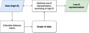
Nada Lavrač: Learning representations for relational learning and literature-based discovery
This was a survey of types of representation learning, focusing on Nada’s area of expertise in propositionalisation and relational data, Bisociative Literature-Based Discovery, and interesting avenues of research in this direction.
Representation Learning
Deep learning, while powerful (accurate), raises concerns over interpretability. Nada takes a step back to survey different forms of representation learning.
Sparse, Symbolic, Propositionalisation:
- These methods tend to be less accurate but are more interpretable.
- Examples include propositionalization techniques that transform relational data into a propositional (flat) format.
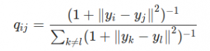
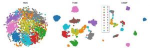
Dense, Embeddings:
- These methods involve creating dense vector representations, such as word embeddings, which are highly accurate but less interpretable.
with recent work focusing on unifying approaches which can incorporate the strengths of both approaches.
Hybrid Methods:
- Incorporate Sparse and Deep methods
- DeepProp, PropDRM, propStar(?) – Methods discussed in their paper.
Representation learning for relational data can be achieved by:
- Propositionalisation – transforming a relational database into a single-table representation. example: Wordification
- Inductive logic programming
- Semantic relational learning
- Relational sub-route discovery (written by Nada and our own P. Flach)
- Semantic subgroup discovery system, “Hedwig” that takes as input the training examples encoded in RDF, and constructs relational rules by effective top-down search of ontologies, also encoded as RDF triples.
- Graph-based machine learning
- data and ontologies are mapped to nodes and edges
- In this example, gene ontologies are used as background knowledge for improving quality assurance of literature-based Gene Ontology Annotation
These slides, although a little out of date, talk about a lot of what I have noted here, plus a few other interesting methodologies.
The GitHub Repo for their book contains lots of jupyter notebook examples.
https://github.com/vpodpecan/representation_learning.git
Marco Gori: Unified approach to learning over time and logic reasoning
I unfortunately found this very difficult to follow, largely due to my lack of subject knowledge. I do think what Marco is proposing requires an open mind as he re-imagines learning systems which do not need to store data to learn, and presents time as an essential component of learning for truly intelligent “Collectionless AI”.
I wont try and rewrite his talk here, but he has full classroom series available on google, which he might give you access to if you email him.
Conclusions:
- Emphasising environmental interactions – collectionless AI which doesn’t record data
- Time is the protagonist: higher degree of autonomy, focus of attention and consciousness
- Learning theory inspired from theoretical physics & optimal control: hamiltonian learning
- Nuero-symbolic learning and reasoning over time: semantic latent fields and explicit semantics
- Developmental stages and gradual knowledge acquisitation
Contacts & Funding Sources
For Robust ML:
e-values, AVCIs:
Aaditya Ramdas at CMU
Peter Grünwald Hiring
For anyone who wants to do a Robust ML PhD, apply to work with Ayush Bharti : https://aalto.wd3.myworkdayjobs.com/aalto/job/Otaniemi-Espoo-Finland/Doctoral-Researcher-in-Statistical-Machine-Learning_R40167
If you know anyone working in edge computing who would like 60K to develop an enterprise solution, here is a link to the funding call: https://daiedge-1oc.fundingbox.com/ The open call starts on 29 August 2024.
If you’d like to receive monthly updates with new funding opportunities from Fundingbox, you can subscribe to their newsletter: https://share-eu1.hsforms.com/1RXq3TNh2Qce_utwh0gnT0wfegdm
Yoshua Bengio said he had fellowship funding but didn’t give out specific details, or I forgot to write them down… perhaps you can send him an email.